Getting started with the API
Chemfp has an extensive Python API. This chapter gives examples of how to use the high-level commands for different types of similarity search, similarity arrays, fingerprint generation and extraction, Butina clustering, and MaxMin and sphere exclusion diversity picking.
Get ChEMBL 34 fingerprints in FPB format
Many of the examples in this section use the RDKit Morgan fingerprints for ChEMBL 32. These are available in FPS format from ChEMBL. I distributed a version in FPB format which includes a chemfp license key to unlock all chemfp functionality for that file.
You will need to download and uncompress that file. Here is one way:
% curl -O https://chemfp.com/datasets/chembl_34.fpb.gz
% gunzip chembl_34.fpb.gz
The FPB file includes the required ChEMBL notices. To see them use:
% chemfp fpb_text chembl_34.fpb
Similarity search of ChEMBL by id
In this section you’ll use the high-level subsearch command to find the closest neighbors to a named fingerprint record.
CHEMBL113 is the ChEMBL record for caffeine.
What are the 5 most similar fingerprints in ChEMBL 32?
Chemfp has several “high-level” functions which provide a lot of
functionality through a single function call. The
chemfp.simsearch() function, like the simsearch command, implements similarity searches.
If given a query id and a target filename then it will open the target fingerprints, find the first fingerprint whose the id matches the query id, and use that fingerprint for a similarity search. When no search parameters are specified, it does a Tanimoto search for the 3 nearest neighbors, which in this case will include CHEMBL113 itself.
>>> import chemfp
>>> result = chemfp.simsearch(query_id="CHEMBL113", targets="chembl_34.fpb")
>>> result
SingleQuerySimsearch('3-nearest Tanimoto search. #queries=1, #targets=2409270
(search: 46.64 ms total: 68.10 ms)', result=SearchResult(#hits=3))
The SingleQuerySimsearch summaries the query and the search
times. In this case it took about 47 milliseconds for the actual
fingerprint search, and 68 milliseconds total; the high-level
organization also has some overhead.
Note
Timings are highly variable. It took 68 ms because the content was in disk cache. With a clear cache it took 210 ms total.
The simsearch result object depends on the type of search. In this case it was a single query vs. a set of targets. The two other supported cases 1) multiple queries against a set of targets, and 2) using the same fingerprints for both targets and queries (a “NxN” search).
The result is a wrapper (really, a proxy) for the underlying search
object, which you can get through result.out:
>>> result.out
SearchResult(#hits=3)
You can access the underlying object directly, but I found myself often forgetting to do that, so the simsearch result objects also implement the underlying search result(s) API, by forwarding them to the actual result, which lets you do things like:
>>> result.get_ids_and_scores()
[('CHEMBL113', 1.0), ('CHEMBL4591369', 0.7333333333333333), ('CHEMBL1232048', 0.7096774193548387)]
As expected, CHEMBL113 is 100% identical to itself. The next closest records are CHEMBL4591369 and CHEMBL1232048.
If you have Pandas installed then use SearchResult.to_pandas()
to export the target id and score to a Pandas Dataframe:
>>> result.to_pandas()
       target_id     score
0      CHEMBL113  1.000000
1  CHEMBL4591369  0.733333
2  CHEMBL1232048  0.709677
The k parameter specifies the number of neighbors to select. The following finds the 10 nearest neighbors and exports the results to a Pandas table using the columns “id” and “Tanimoto”:
>>> chemfp.simsearch(query_id="CHEMBL113",
...      targets="chembl_34.fpb", k=10).to_pandas(columns=["id", "Tanimoto"])
              id  Tanimoto
0      CHEMBL113  1.000000
1  CHEMBL4591369  0.733333
2  CHEMBL1232048  0.709677
3   CHEMBL446784  0.677419
4  CHEMBL1738791  0.666667
5  CHEMBL2058173  0.666667
6   CHEMBL286680  0.647059
7   CHEMBL417654  0.647059
8  CHEMBL2058174  0.647059
9  CHEMBL1200569  0.641026
Similarity search of ChEMBL using a SMILES
In this section you’ll use the high-level subsearch command to find target fingerprints which are at least 0.75 similarity to a given SMILES string. The next section will show how to sort by score.
Wikipedia gives
O=C(NCc1cc(OC)c(O)cc1)CCCC/C=C/C(C)C as a SMILES for
capsaicin. What ChEMBL structures are at leat 0.75 similar to that
SMILES?
The chemfp.simsearch() function supports many types of query
inputs. The previous section used used a query id to look up the
fingerprint in the targets. Alternatively, the query parameter
takes a string containing a structure record, by default in “smi”
format. (Use query_format to specify “sdf”, “molfile”, or other
supported format.):
>>> import chemfp
>>> result = chemfp.simsearch(query = "O=C(NCc1cc(OC)c(O)cc1)CCCC/C=C/C(C)C",
...     targets="chembl_34.fpb", threshold=0.75)
>>> len(result)
23
>>> result.to_pandas()
        target_id     score
0   CHEMBL4227443  0.791667
1     CHEMBL87171  0.795918
2     CHEMBL76903  0.764706
3     CHEMBL80637  0.764706
4     CHEMBL86356  0.764706
5     CHEMBL88024  0.764706
6     CHEMBL87024  0.764706
7     CHEMBL89699  0.764706
8     CHEMBL88913  0.764706
9     CHEMBL89176  0.764706
10    CHEMBL89356  0.764706
11    CHEMBL89829  0.764706
12   CHEMBL121925  0.764706
13   CHEMBL294199  1.000000
14   CHEMBL313971  1.000000
15   CHEMBL314776  0.764706
16   CHEMBL330020  0.764706
17   CHEMBL424244  0.764706
18  CHEMBL1672687  0.764706
19  CHEMBL1975693  0.764706
20  CHEMBL3187928  1.000000
21    CHEMBL88076  0.750000
22   CHEMBL313474  0.750000
The next section will show how to sort the results by score.
Sorting the search results
The previous section showed how to find all ChEMBL fingerprints with 0.75 similarity to capsaicin. This section shows how to sort the scores in chemfp, which is faster than using Pandas to sort.
While chemfp’s k-nearest search orders the hits from highest to
lowest, the threshold search order is arbitrary (or more precisely,
based on implementation-specific factors). If you want sorted scores
in the Pandas table you could do so using Pandas’ sort_values
method, as in the following:
>>> chemfp.simsearch(query = "O=C(NCc1cc(OC)c(O)cc1)CCCC/C=C/C(C)C",
...     targets="chembl_34.fpb", threshold=0.75).to_pandas().sort_values("score", ascending=False)
        target_id     score
20  CHEMBL3187928  1.000000
14   CHEMBL313971  1.000000
13   CHEMBL294199  1.000000
1     CHEMBL87171  0.795918
0   CHEMBL4227443  0.791667
19  CHEMBL1975693  0.764706
18  CHEMBL1672687  0.764706
17   CHEMBL424244  0.764706
16   CHEMBL330020  0.764706
15   CHEMBL314776  0.764706
12   CHEMBL121925  0.764706
11    CHEMBL89829  0.764706
10    CHEMBL89356  0.764706
9     CHEMBL89176  0.764706
8     CHEMBL88913  0.764706
7     CHEMBL89699  0.764706
6     CHEMBL87024  0.764706
5     CHEMBL88024  0.764706
4     CHEMBL86356  0.764706
3     CHEMBL80637  0.764706
2     CHEMBL76903  0.764706
21    CHEMBL88076  0.750000
22   CHEMBL313474  0.750000
However, it’s a bit faster to have chemfp sort the results before exporting to Pandas. (For a large data set, about 10x faster.)
The simsearch ordering parameter takes one of the following
strings:
“increasing-score” - sort by increasing score
“decreasing-score” - sort by decreasing score
“increasing-score-plus” - sort by increasing score, break ties by increasing index
“decreasing-score-plus” - sort by decreasing score, break ties by increasing index
“increasing-index” - sort by increasing target index
“decreasing-index” - sort by decreasing target index
“move-closest-first” - move the hit with the highest score to the first position
“reverse” - reverse the current ordering
Here’s how order the simsearch results by “decreasing-score”:
>>> chemfp.simsearch(query = "O=C(NCc1cc(OC)c(O)cc1)CCCC/C=C/C(C)C",
...     targets="chembl_34.fpb", threshold=0.75, ordering="decreasing-score").to_pandas()
        target_id     score
0    CHEMBL294199  1.000000
1    CHEMBL313971  1.000000
2   CHEMBL3187928  1.000000
3     CHEMBL87171  0.795918
4   CHEMBL4227443  0.791667
5     CHEMBL76903  0.764706
6     CHEMBL80637  0.764706
7     CHEMBL86356  0.764706
8     CHEMBL88024  0.764706
9     CHEMBL87024  0.764706
10    CHEMBL89699  0.764706
11    CHEMBL88913  0.764706
12    CHEMBL89176  0.764706
13    CHEMBL89356  0.764706
14    CHEMBL89829  0.764706
15   CHEMBL121925  0.764706
16   CHEMBL314776  0.764706
17   CHEMBL330020  0.764706
18   CHEMBL424244  0.764706
19  CHEMBL1672687  0.764706
20  CHEMBL1975693  0.764706
21    CHEMBL88076  0.750000
22   CHEMBL313474  0.750000
Fingerprints as byte strings
In this section you’ll learn how chemfp uses byte strings to represent a fingerprint.
Chemfp works with binary fingerprints, typically in the range of a few hundred to a few thousand bits, and with a bit density high enough that sparse representations aren’t useful.
There are several common ways to represent these fingerprints. Chemfp uses a byte string, including at the Python level. (Two common alternatives are to have detected “fingerprint object”, or to re-use something like Python’s arbitrary-length integers.)
Here, for example, is a 24-bit fingerprint in Python:
>>> fp = b"XYZ"
The leading ‘b’ indicates the string is a byte string.
Remember, normal Python strings (also called Unicode strings) are different from byte strings. Byte strings are a sequence of 8-bits values, while normal strings use a more complicated representation that can handle the diversity of human language.
Chemfp includes functions in the bitops module to work with byte-string fingerprints. For example, here are the positions of the on-bits in the fingerprint:
>>> from chemfp import bitops
>>> bitops.byte_to_bitlist(b"XYZ")
[3, 4, 6, 8, 11, 12, 14, 17, 19, 20, 22]
>>> bitops.byte_to_bitlist(b"ABC")
[0, 6, 9, 14, 16, 17, 22]
and here is the Tanimoto between those two byte strings:
>>> bitops.byte_tanimoto(b"ABC", b"XYZ")
0.2857142857142857
You can verify they share bits 6, 14, 17, and 22, while the other 10 bits are distinct, giving a Tanimoto of 4/14 = 0.2857142857142857.
If you are working with hex-encoded fingerprints then you can use Python’s bytestring methods to convert to- and from- those values:
>>> b"ABC".hex()
'414243'
>>> bytes.fromhex("4101ff")
b'A\x01\xff'
Python’s fromhex() does not accept a byte string:
>>> bytes.fromhex(b"4101ff")
Traceback (most recent call last):
  File "<stdin>", line 1, in <module>
TypeError: fromhex() argument must be str, not bytes
If you have a byte string you might consider using chemfp’s
hex_decode() function, which supports both types of strings:
>>> bitops.hex_decode("4101ff")
b'A\x01\xff'
>>> bitops.hex_decode(b"4101ff")
b'A\x01\xff'
or use one of the “hex” functions in the bitops module, which work on hex-encoded fingerprints:
>>> bitops.hex_to_bitlist("4101ff")
[0, 6, 8, 16, 17, 18, 19, 20, 21, 22, 23]
>>> bitops.byte_to_bitlist(b"A\x01\xff")
[0, 6, 8, 16, 17, 18, 19, 20, 21, 22, 23]
Generating Fingerprints
In this section you’ll learn how to generate a fingerprint using chemfp’s interface to several supported cheminformatics toolkits.
Chemfp is a package for working with cheminformatics fingerprints. It is not a cheminformatics toolkit. It instead knows how to use OpenEye’s OEChem and OEGraphSim, the RDKit, Open Babel, and CDK to read and write molecules, and to generate fingerprints.
I’ll use the MACCS fingerprints in this section because they are a well-known fingerprint with a long history in this field, they implemented in all of the supported toolkits, and they are short enough to include in the documentation. However:
Important
Do not use the MACCS fingerprints in modern research. They are only of historical interest.
In chemfp, a FingerprintType describes an object which can
generate fingerprints, typically from a structure record. These know
what kind of fingerprints to generate (eg, “MACCS” or “circular”;
chemfp calls this a “fingerprint family”), as well as any
configuration parameters (eg, fingerprint size, radius, and atom type
flags).
Each of chemfp’s toolkit interfaces includes several FingerprintTypes, one for the toolkit’s fingerprint types, using the default parameters, if any. Here are the ones for the MACCS keys:
>>> import chemfp
>>> chemfp.rdkit.maccs166
RDKitMACCSFingerprintType_v2(<RDKit-MACCS166/2>)
>>> chemfp.openbabel.maccs
OpenBabelMACCSFingerprintType_v2(<OpenBabel-MACCS/2>)
>>> chemfp.cdk.maccs
CDKMACCSFingerprintType_v20(<CDK-MACCS/2.0>)
>>> chemfp.openeye.maccs166
OpenEyeMACCSFingerprintType_v3(<OpenEye-MACCS166/3>)
Chemfp’s choice of “maccs” vs “maccs166” follows the naming convention of the underlying toolkit.
The fingerprint types subclasses implement from_smiles which takes
a SMILES string, uses the underlying toolkit to parse the SMILES into
a toolkit molecule and generate a fingerprint, and returns the
fingerprint as a byte string.:
>>> import chemfp
>>> chemfp.rdkit.maccs166.from_smiles("Cn1cnc2c1c(=O)[nH]c(=O)n2C")
b'\x00\x00\x00\x000\x00\x00\x00\x01\xd4\x14\xd9\x13#\x91S\x80\xe1x\xea\x1f'
>>> chemfp.openbabel.maccs.from_smiles("Cn1cnc2c1c(=O)[nH]c(=O)n2C")
b'\x00\x00\x00\x000\x00\x00\x00\x01\xd4\x14\xd9\x13#\x91C\x80\xe1x\xea\x1f'
>>> chemfp.cdk.maccs.from_smiles("Cn1cnc2c1c(=O)[nH]c(=O)n2C")
b'\x00\x00\x00\x000\x00\x00\x00\x01\xd4\x14\xd9\x03#\x91C\x80\xe1x\xea\x1f'
>>> chemfp.openeye.maccs166.from_smiles("Cn1cnc2c1c(=O)[nH]c(=O)n2C")
b'\x00\x00\x00\x000\x00\x00\x00\x01\xd4\x14\xd9\x13\xa3\x91C\x80\xa0zj\x1b'
What’s the difference between the RDKit and Open Babel or CDK
fingerprints? I’ll use byte_to_bitlist() to get the bits in each
one, then use Python’s set algebra to see which bits are set in one but no the other:
>>> from chemfp import bitops
>>> set(bitops.byte_to_bitlist(rd_maccs)) - set(bitops.byte_to_bitlist(ob_maccs))
{124}
>>> set(bitops.byte_to_bitlist(ob_maccs)) - set(bitops.byte_to_bitlist(rd_maccs))
set()
>>> set(bitops.byte_to_bitlist(rd_maccs)) - set(bitops.byte_to_bitlist(cdk_maccs))
{124, 100}
>>> set(bitops.byte_to_bitlist(cdk_maccs)) - set(bitops.byte_to_bitlist(rd_maccs))
set()
Some toolkits store MACCS key 1 in bit 0 (the first bit) and others store key 1 in bit 1, leaving bit 0 empty. Chemfp’s standardizes all MACCS fingerprints to start at bit 0.
Similarity Search of ChEMBL by fingerprint
In this section you’ll learn how to search ChEMBL using a fingerprint byte string as the query.
ChEMBL generated the ChEBML fingerprints using RDKit’s Morgan fingerprints with the default settings. The corresponding chemfp fingerprint type string is:
RDKit-Morgan/1 radius=2 fpSize=2048 useFeatures=0 useChirality=0 useBondTypes=1
This is version 1 of the Morgan fingerprints, with a radius of 2. It generates 2048-bit fingerprints. This is an ECFP-like circular fingerprint because the atom invariants were used rather than the FCFP-like version using feature invariants. Chirality was not included in the generation method, while bond type were considered.
The version number is there to reflect changes in the underlying algorithm or API. In this case, version 1 means it uses RDKit’s older function-based API. Chemfp 4.2 introduced a version 2 Morgan fingerprint type based on RDKit’s newer generator API, which uses different parameters. Chemfp currently supports both fingerprint types.
If you know this type string, you can use chemfp’s
chemfp.get_fingerprint_type() function to parse the string and return
the appropriate FingerprintType object, then parse a SMILES and get
its fingerprint:
>>> import chemfp
>>> fptype = chemfp.get_fingerprint_type(
...    "RDKit-Morgan/1 radius=2 fpSize=2048 useFeatures=0 useChirality=0 useBondTypes=1")
>>> fptype
RDKitMorganFingerprintType_v1(<RDKit-Morgan/1 radius=2 fpSize=2048 useFeatures=0 useChirality=0 useBondTypes=1>)
>>> fp = fptype.from_smiles("Cn1cnc2c1c(=O)[nH]c(=O)n2C")
>>> fp[:10] + b" ... " + fp[-10:]
b'\x00\x00\x00\x00\x02\x00\x00\x02\x00\x00 ... \x00\x00\x00\x00\x00\x00\x00\x00\x00\x00'
Alternatively you can use the default Morgan2 v1 fingerprint type from
the rdkit_toolkit module, available through the
chemfp.rdkit helper:
>>> fp = chemfp.rdkit.morgan2_v1.from_smiles("Cn1cnc2c1c(=O)[nH]c(=O)n2C")
Use query_fp to have chemfp.simsearch() search using the
given fingerprint as a query:
>>> chemfp.simsearch(query_fp=fp, targets="chembl_34.fpb", k=4).to_pandas()
       target_id     score
0     CHEMBL1114  1.000000
1  CHEMBL2106653  0.794118
2   CHEMBL131371  0.638889
3  CHEMBL2107523  0.613636
Load fingerprints into an arena
In this section you’ll learn about chemfp’s fingerprint “arena”, and how to load one from a fingerprint file.
The fastest way for chemfp to do a similarity search is to load all of
the fingerprints in memory in a data struture called an “arena”. Use
the chemfp.load_fingerprints() command to read an FPS or FPB file into
an arena, like this:
>>> import chemfp
>>> arena1 = chemfp.load_fingerprints("chembl_34.fps.gz")
>>> arena2 = chemfp.load_fingerprints("chembl_34.fpb")
If you do those steps you’ll see arena1 takes about 10 seconds to load, while arena2 takes well less than a second.
There’s a very straight-forward explanation. Chemfp must decompress and parse the fps.gz file and arrange the content into an arena, while the fpb file is internally already structured as an arena, so requires little additional processing.
What’s in an arena? Here’s the Python representation of both arenas, and a few operations on arena2:
>>> arena1
FingerprintArena(#fingerprints=2409270)
>>> arena2
FPBFingerprintArena(#fingerprints=2409270)
>>> len(arena2)
2409270
>>> arena2.get_index_by_id("CHEMBL113")
41028
>>> arena2.ids[41028]
'CHEMBL113'
>>> arena2.fingerprints[41028][:16]
b'\x00\x00\x00\x00\x02\x00\x00\x00\x00\x00\x00\x00\x00\x00\x00\x00'
>>> arena2[41028]
('CHEMBL113', b'\x00\x00\x00\x00\x02\x00\x00\x00\x00\x00
\x00\x00\x00\x00\x00\x00\x00\x00\x00\x00\x00\x00\x00\x00
\x00\x00\x00\x00\x00\x00\x00\x00\x00\x00\x00\x00\x00\x00
 ... many lines removed ...
>>> arena2.fingerprints.random_choice()[:8]
b'\x02\x00\x00\x00\x00@\x00\x01'
The main difference between a FingerprintArena and an
FPBFingerprintArena is the FPBFingerprintArena uses a
memory-mapped to access the file contents, which means it as an open
file handle. Use close method or a context manager if you don’t want
to depend on Python’s garbage collector to close the file. (The
FingerprintArena also implements close, which does nothing.)
The FPS and FPB files may store the fingerprint type string as metadata, which is available from the arena:
>>> import chemfp
>>> arena = chemfp.load_fingerprints("chembl_34.fpb")
>>> arena.metadata.type
'RDKit-Morgan/1 radius=2 fpSize=2048 useFeatures=0 useChirality=0 useBondTypes=1'
Use the arena’s FingerprintReader.get_fingerprint_type() method
to get corresponding FingerprintType object:
>>> arena.get_fingerprint_type()
RDKitMorganFingerprintType_v1(<RDKit-Morgan/1 radius=2 fpSize=2048
useFeatures=0 useChirality=0 useBondTypes=1>)
The arena has some other useful methods, like ways to get the total
number of 1 bits set for each bit position, using
FingerprintArena.get_bit_counts() for a Python array, or
FingerprintArena.get_bit_counts_as_numpy() for a NumPy array:
>>> arena.get_bit_counts()[:10]
array('i', [8217, 577135, 118848, 16329, 42582, 74983, 9011, 21002, 64433, 50386])
>>> arena.get_bit_counts_as_numpy()[:10]
array([  8217, 577135, 118848,  16329,  42582,  74983,   9011,  21002,
        64433,  50386], dtype=int32)
or to generate random subset with FingerprintArena.sample() :
>>> subset1 = arena.sample(100)  # 100 elements
>>> subset2 = arena.sample(0.01)  # 1% of the full set
>>> len(subset2)
24092
or to generate two random and non-overlapping subsets with
FingerprintArena.train_test_split():
>>> train, test = arena.train_test_split(train_size=100, test_size=0.005)
>>> len(train), len(test)
(100, 12046)
Both the sample and train_test_split methods are modelled after
the equivalent ones in scikit-learn.
Lastly, the FingerprintArena.to_numpy_array()
returns a NumPy view of the underlying data as unsigned bytes (this
should have been named “as_numpy_array”):
>>> arena.to_numpy_array()
array([[ 0,  0,  0, ...,  0,  0,  0],
       [ 0,  0,  0, ...,  0,  0,  0],
       [ 0,  0,  0, ...,  0,  0,  0],
       ...,
       [34, 33,  0, ...,  4,  2,  8],
       [34,  0, 12, ...,  0,  0,  4],
       [34,  0,  8, ...,  0,  0,  4]], dtype=uint8)
>>> arena.to_numpy_array().shape
(2409270, 256)
and FingerprintArena.to_numpy_bitarray() returns a new NumPy
array with a single uint8 value for each bit position:
>>> arena.to_numpy_bitarray()
array([[0, 0, 0, ..., 0, 0, 0],
       [0, 0, 0, ..., 0, 0, 0],
       [0, 0, 0, ..., 0, 0, 0],
       ...,
       [0, 1, 0, ..., 0, 0, 0],
       [0, 1, 0, ..., 0, 0, 0],
       [0, 1, 0, ..., 0, 0, 0]], dtype=uint8)
>>> arena.to_numpy_bitarray().shape
(2409270, 2048)
Generate an NxN similarity matrix
In this section you’ll learn how to do an NxN search with
chemfp.simsearch(), using an arena as both the queries and the
targets.
The simsearch examples in the previous sections all took an FPB filename for the targets, which means the function had to open the file each time. You can also use an arena as the targets, which is useful if you will be doing many searches.:
>>> import chemfp
>>> arena = chemfp.load_fingerprints("chembl_34.fpb")
>>> chemfp.simsearch(query_id="CHEMBL1114", targets=arena, k=2).to_pandas()
       target_id     score
0     CHEMBL1114  1.000000
1  CHEMBL2106653 0.794118
>>> chemfp.simsearch(query_id="CHEMBL2106653", targets=arena, k=2).to_pandas()
       target_id     score
0  CHEMBL2106653  1.000000
1     CHEMBL1114  0.794118
(This means theobromine and theobromine sodium acetate are both each other’s nearest neighbors.)
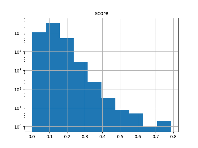
It’s also useful when working with subsets. The following selects 1000 fingerprints at random (using a specified seed for reproducibility), computes the N*(N-1)/2 upper-triangle similarity matrix of all pairwise comparisons, and generates a histogram of the scores:
>>> subset = arena.sample(1000, rng=87501)
>>> subset
FingerprintArena(#fingerprints=1000)
>>> ut = chemfp.simsearch(targets=subset, NxN=True,
...   threshold=0.0, include_lower_triangle=False)
queries: 100%|█████████████████████| 1000/1000 [00:00<00:00, 57873.22 fps/s]
>>> from matplotlib import pyplot as plt
>>> ut.to_pandas().hist("score", log=True)
If you are in the Jupyter notebook then you should see the following image:
If you are in the traditional Python shell then to see the image you’ll also need to do:
>>> from matplotlib import pyplot as plt
>>> plt.show()
Note
chemfp’s NxN search is designed for a sparse result matrix. While it can certainly be used to compute all pairwise comparisons, it will not be as fast as simarray, which was designed for that purpose.
The NxN search displays a progress bar by default. If you do not want
a progress bar, either pass progress = False to simsearch, or
globally disable the use of the default progress bar with:
>>> chemfp.set_default_progressbar(False)
To re-enable it, use:
>>> chemfp.set_default_progressbar(True)
Generate an NxM similarity matrix
In this section you’ll learn how to use multiple queries to search a
set of target fingerprints using chemfp.simsearch().
Earlier you learned several ways to search the ChEMBL fingerprints
using a single query. If you have multiple queries then use the
queries parameter to pass a query arena to simsearch.
For example, given two fingerprint sets A and B, which fingerprint in A is closest to a fingerprint in B?
To make it a bit more interesting, I’ll let A be the first 1,000 ChEMBL records and B be the last 1,000 ChEMBL records, sorted by id, on the assumption they are roughly time-ordered.
The identifiers are available from the id attribute, but these are either in popcount order (the default) or input order.
Tip
“Popcount”, which is short for “population count”, is the number of 1-bits in the fingerprint
Here are a few examples. They show that id is a list-like object, and that the fingerprints of the first and last identifiers have very different popcounts:
>>> import chemfp
>>> arena = chemfp.load_fingerprints("chembl_34.fpb")
>>> arena.ids
IdLookup(<695649856 bytes>, #4=2409270, #8=0, data_start=616781600, index_start=647462380)
>>> arena.ids[:2]
IdLookup(<695649856 bytes>, #4=2, #8=0, data_start=616781600, index_start=647462380)
>>> list(arena.ids[:2])  # the first two ids
['CHEMBL17564', 'CHEMBL4300465']
>>> list(arena.ids[-2:])  # the last two ids
['CHEMBL5314953', 'CHEMBL5219064']
>>>
>>> from chemfp import bitops
>>> bitops.byte_popcount(arena.get_fingerprint_by_id("CHEMBL17564"))
1
>>> bitops.byte_popcount(arena.get_fingerprint_by_id("CHEMBL5219064"))
249
We can’t simply sort by id because the default string sort places “CHEMBL10” before “CHEMBL2”. Instead, we need to remove the leading “CHEMBL”, convert the rest to an integer, and then do the sort.
I’ll start with a function to remove the first 6 characters and convert the rest to an integer:
def get_serial_number(s):
    return int(s[6:])
I’ll use that to sort all of the identifiers by serial number:
>>> sorted_ids = sorted(arena.ids, key = get_serial_number)
>>> sorted_ids[:3]
['CHEMBL1', 'CHEMBL2', 'CHEMBL3']
>>> sorted_ids[-3:]
['CHEMBL5316226', 'CHEMBL5316227', 'CHEMBL5316228']
Seems to work!
Next, I’ll make subsets A and B using the
FingerprintArena.copy() method, which if passed a list of
indices will make a copy of only that subset:
>>> subset_A = arena.copy(
...   indices=[arena.get_index_by_id(id) for id in sorted_ids[:1000]])
>>> subset_B = arena.copy(
...   indices=[arena.get_index_by_id(id) for id in sorted_ids[-1000:]])
Now for the similarity search step. I’ll do a k=1 nearest-neighbor search for each fingerprint in A to find its closest match in B:
>>> result = chemfp.simsearch(queries=subset_A, targets=subset_B, k=1)
queries: 100%|████████████████████| 1000/1000 [00:00<00:00, 33987.02 fps/s]
>>> result
MultiQuerySimsearch('1-nearest Tanimoto search. #queries=1000, #targets=1000
(search: 30.99 ms total: 34.27 ms)', result=SearchResults(#queries=1000, #targets=1000))
There are a few ways to find the hit with the highest score. One uses standard Python, but I need to explain the details.
The MultiQuerySimsearch object, just like the underlying
SearchResults object, implements index lookup, so I’ll focus
on the first hit:
>>> first_hit = result[0]
>>> first_hit
SearchResult(#hits=1)
The SearchResult object knows the initial query id and has
ways to get the target indices, ids, and scores for the hits:
>>> first_hit.query_id
'CHEMBL1141'
>>> first_hit.get_ids_and_scores()
>>> first_hit.get_ids_and_scores()
[('CHEMBL5315938', 0.030303030303030304)]
>>> first_hit.get_scores()
array('d', [0.030303030303030304])
With a slightly clumsy list comprehension, here’s the highest scoring pair:
>>> max((hits.get_scores()[0], hits.query_id, hits.get_ids()[0]) for hits in result)
(0.6875, 'CHEMBL1069', 'CHEMBL5315276')
Alternatively, use Pandas:
>>> result.to_pandas().nlargest(1, columns="score")
       query_id      target_id   score
895  CHEMBL1069  CHEMBL5315276  0.6875
along with a quick check for ties:
>>> result.to_pandas().nlargest(5, columns="score")
       query_id      target_id     score
895  CHEMBL1069  CHEMBL5315276  0.687500
955   CHEMBL941  CHEMBL5316157  0.681818
443    CHEMBL56  CHEMBL5315307  0.659574
681   CHEMBL560  CHEMBL5316208  0.654545
598   CHEMBL118  CHEMBL5315305  0.625000
No wonder people enjoy using Pandas!
Before leaving this section, I’ll also show an advanced technique to get the fingerprint indices sorted by serial number, without doing the id-to-index lookup:
>>> serial_numbers = [get_serial_number(id) for id in arena.ids]
>>> sorted_indices = sorted(range(len(serial_numbers)),
...    key = serial_numbers.__getitem__)
>>> arena.ids[sorted_indices[0]]
'CHEMBL1'
>>> arena.ids[sorted_indices[-1]]
'CHEMBL5316228'
>>> subset_A = arena.copy(indices=sorted_indices[:100])
>>> subset_B = arena.copy(indices=sorted_indices[-100:])
I’ll leave this one as a puzzler, which it was to me the first time I came across it.
Exporting SearchResults to SciPy and NumPy
In this section you’ll learn how to use convert chemfp’s
SearchResults object to a SciPy sparse array and to a NumPy
dense array.
Chemfp uses its own data structure to store similarity search results,
which is available to Python as a SearchResults
instance. This implements a sparse row array where each row stores the
target ids and Tanimoto/Tversky scores, along with some methods to
access that data.
The following generates two small randomly selected subsets from ChEMBL 34 and generates the NxM comparison matrix between the two, with a minimum threshold of 0.2:
>>> import chemfp
>>> arena = chemfp.load_fingerprints("chembl_34.fpb")
>>> train, test = arena.train_test_split(300, 1250, rng=321)
>>> len(train), len(test)
(300, 1250)
>>> result = chemfp.simsearch(queries=train, targets=test,
...    threshold=0.2, progress=False)
>>> result.count_all()
9897
>>> 300*1250
375000
>>> result[278]
SearchResult(#hits=3)
>>> result[278].get_scores()
array('d', [0.22115384615384615, 0.3333333333333333, 0.2627118644067797])
>>> result[278].get_indices()
array('i', [812, 824, 1184])
>>> result[278].get_ids_and_scores()
[('CHEMBL1992753', 0.22115384615384615), ('CHEMBL553600',
0.3333333333333333), ('CHEMBL2011810', 0.2627118644067797)]
Even with the low threshold of 0.2 only 2.6% of the comparisons are at or above it, which is why chemfp uses a sparse representation.
While all of the data is accessible through chemfp’s Python API, there are not many analysis tools which understand that API, and there isn’t a high-performance way for C code to access the entire array.
Instead, you can export the search results to a SciPy “csr” (compressed sparse row matrix):
>>> csr = result.to_csr()
>>> csr[278]
<1x1250 sparse matrix of type '<class 'numpy.float64'>'
      with 3 stored elements in Compressed Sparse Row format>
These are indexed in the same coordinate system as the original search results:
>>> csr[278]
<1x1250 sparse matrix of type '<class 'numpy.float64'>'
      with 3 stored elements in Compressed Sparse Row format>
>>> csr[278].data
array([0.22115385, 0.33333333, 0.26271186])
>>> csr[278].indices
array([ 812,  824, 1184], dtype=int32)
>>> csr[278, 812]
0.22115384615384615
>>> result.target_ids[812]
'CHEMBL1992753'
Alternatively, you can export the search results to a (dense) NumPy array, which uses 0.0 for all missing entries:
>>> arr = result.to_numpy_array()
>>> arr[:3, :4]
array([[0.        , 0.        , 0.        , 0.        ],
       [0.        , 0.        , 0.        , 0.        ],
       [0.29166667, 0.        , 0.        , 0.        ]])
>>> arr[278]
array([0., 0., 0., ..., 0., 0., 0.])
>>> arr[278].nonzero()
(array([ 812,  824, 1184]),)
Both to_csr and to_numpy_array let you specify the NumPy data type as
dtype="float64" or dtype="float32"; with float64 as the
default, as that matches chemfp’s own internal representation.
You can also compute the full NumPy array directly using
chemfp.simarray(), as shown below.
Note
A symmetric simsearch does not contain the diagonals
By design simarray, for NxN symmetric search, does not compare a fingerprint with itself, which means the sparse and dense arrays will be zero along the diagonal:
>>> full = chemfp.simsearch(targets=train, NxN=True, threshold=0.0)
queries: 100%|███████████████████████████| 300/300 [00:00<00:00, 28131.44 fps/s]
>>> arr = full.to_numpy_array()
>>> arr[:3, :3]
array([[0.        , 0.05263158, 0.05      ],
       [0.05263158, 0.        , 0.03846154],
       [0.05      , 0.03846154, 0.        ]])
If you need the diagonals to be 1.0 then you will need to modify it yourself, such as the following:
>>> arr += numpy.identity(len(train))
>>> arr[:3, :3]
array([[1.        , 0.05263158, 0.05      ],
       [0.05263158, 1.        , 0.03846154],
       [0.05      , 0.03846154, 1.        ]])
Save simsearch results to an npz file
In this section you’ll learn how to save a simsearch result to a NumPy npz file, formatted for use as
an SciPy csr array. You’ll also learn how chemfp stores metadata and
identifiers in the array, so it can be loaded back into a chemfp
SearchResults for later use.
The chemfp simsearch results can be saved to NumPy “npz” format using
SearchResults.save():
>>> import chemfp
>>> arena = chemfp.load_fingerprints("chembl_34.fpb")
>>> train, test = arena.train_test_split(300, 1250, rng=321)
>>> result = chemfp.simsearch(queries=train, targets=test,
...    threshold=0.2, progress=False)
>>> result.save("my_data.npz")
The npz format is a zipfile containing NumPy arrays formatted in “npy” format. I’ll use Python’s built-in zipfile module to show the contents, so you can see how it works - use a method below to actually access the data:
>>> import zipfile
>>> z = zipfile.ZipFile("my_data.npz")
>>> ['chemfp.npy', 'indices.npy', 'indptr.npy', 'format.npy',
'shape.npy',  'data.npy', 'query_ids.npy', 'target_ids.npy']
SciPy saves sparse arrays to npz format using entries following a special naming convention, where the files “format.npy”, “shape.npy”, “indices.npy”, “indptr.npy”, and “data.npy” all have special meaning. For examples, “format.npy” describes the type of SciPy sparse array, and the “shape.npy” describes its shape:
>>> import numpy
>>> numpy.load(z.open("format.npy"))
array('csr', dtype='<U3')
>>> numpy.load(z.open("shape.npy"))
array([ 300, 1250])
Use SciPy’s load_npz
function to load the data into a SciPy csr array, or use chemfp’s own
load_npz function (described in a few
paragraphs) to load it into a chemfp SearchResult or
SearchResults. Here’s an example using SciPy:
>>> import scipy.sparse
>>> csr = scipy.sparse.load_npz("my_data.npz")
>>> csr
<300x1250 sparse matrix of type '<class 'numpy.float64'>'
      with 9897 stored elements in Compressed Sparse Row format>
>>> csr[278, 812]
0.22115384615384615
Chemfp adds two or three more npz entries, depending on the type of search. The “chemfp.npy” file contains a NumPy array with a JSON-encoded string describing the search parameters. In this case, with an NxM search, the “query_ids.npy” file contain the query identifiers, and the “target_ids.npy” file contain the target identifiers:
>>> query_ids = numpy.load(z.open("query_ids.npy"))
>>> target_ids = numpy.load(z.open("target_ids.npy"))
>>> query_ids[278]
'CHEMBL17529'
>>> target_ids[812]
'CHEMBL1992753'
For a symmetric/NxN search, or for a single query search against a set of targets where there are only target ids, the “ids.npy” entry stores the relevant identifiers.
Chemfp’s own chemfp.search.load_npz() will load the npz file
and return a SearchResults for a 2-D result, or a
SearchResult for single query searches. This includes
loading the query and target identifiers:
>>> import chemfp.search
>>> results = chemfp.search.load_npz("my_data.npz")
>>> result[278].query_id
'CHEMBL17529'
>>> result[278].get_ids_and_scores()
[('CHEMBL1992753', 0.22115384615384615), ('CHEMBL553600',
0.3333333333333333), ('CHEMBL2011810', 0.2627118644067797)]
Use simarray to generate a NumPy array
In this section you’ll learn how to use chemfp.simarray() to
generate a NumPy array containing all of the fingerprint pairwise
comparisons. (See Generate a full Tanimoto similarity array for an example using
the chemfp simarray command-line tool.)
Many algorithms, like some of the sckit-learn clustering methods,
require the complete NxN comparisons between every element and every
other element, including with itself, as a NumPy array. While this is
possible with chemfp.simsearch(), by using a threshold of 0.0
then converting it into NumPy array, and setting the diagonal terms to
1.0, it’s cumbersome and inefficient.
Instead, use chemfp.simarray(). The following selects 20,000
fingerprints at random from ChEMBL 34 then computes the 400 million
Tanimoto scores in about 3 seconds:
>>> import chemfp
>>> arena = chemfp.load_fingerprints("chembl_34.fpb")
>>> subset = arena.sample(20_000, rng=987, reorder=False)
>>> simarr = chemfp.simarray(targets=subset)
scores: 100%|█████████████████████████████████| 200M/200M [00:03<00:00, 63.3M/s]
>>> simarr.out[:4, :4]
array([[1.        , 0.20512821, 0.128     , 0.11702128],
       [0.20512821, 1.        , 0.12903226, 0.11827957],
       [0.128     , 0.12903226, 1.        , 0.14285714],
       [0.11702128, 0.11827957, 0.14285714, 1.        ]])
The reorder=False is there so the subset is in random order,
rather than the default of sorting the new subset by
popcount. Simarray performance, unlike simsearch performance, does not
benefit from reordering, and the 4x4 corner of the sorted subset is a
poor example as the sparse fingerprints cause that region to look like
the identify matrix.
The returned SimarrayResult contains the NumPy array in the
out attribute, along with other information related to the
search. Its repr summarizes the details:
>>> simarr
SimarrayResult(metric=<Tanimoto similarity>, out=<20000x20000
symmetric array of dtype float64>, query_ids=target_ids=['CHEMBL3646927',
'CHEMBL3643396', 'CHEMBL4111145', ...], times=<process: 3.16 s, total: 3.16 s>)
This says it computed Tanimoto similarities, stored in a 20,000 by 20,000 symmetric array of float64 values. Because it’s a symmetric search, the query and target ids are the same, and it shows the first three of them. Finally, it took 3.16s to generate the results.
Unlike simsearch, which only implements
Tanimoto and the more generalized Tversky search, both stored as
float64 values, simarray has built-in
support for a few other comparison methods and data types.
For example, instead of the Tanimoto similarity (also called the
Jaccard similarity) do you want the Jaccard distance, computed as
1-Tanimoto? Use the as_distance parameter:
>>> distarr = chemfp.simarray(targets=subset, as_distance=True)
scores: 100%|█████████████████████████████████| 200M/200M [00:02<00:00, 67.5M/s]
>>> distarr.out[:3, :3]
array([[0.        , 0.79487179, 0.872     ],
       [0.79487179, 0.        , 0.87096774],
       [0.872     , 0.87096774, 0.        ]])
This calculation is slightly more accurate than computing
1-simarr.out because the Jaccard distance is computed as a rational
first, before the divison, while the subtraction from 1.0 introduces a
potential rounding error:
>>> distarr.out[:3, :3] == 1-simarr.out[:3, :3]
array([[ True, False,  True],
       [False,  True,  True],
       [ True,  True,  True]])
>>> 1-simarr.out[:3, :3] - distarr.out[:3, :3]
array([[0.00000000e+00, 1.11022302e-16, 0.00000000e+00],
       [1.11022302e-16, 0.00000000e+00, 0.00000000e+00],
       [0.00000000e+00, 0.00000000e+00, 0.00000000e+00]])
Perhaps you want the cosine similarity (use metric="cosine"), with
the results stored in a float32 (use dtype="float32"), which only
only needs half the space as float64?
>>> simarr = chemfp.simarray(targets=subset, metric="cosine",
...   dtype="float32", progress=False)
>>> simarr.get_description(include_times=False)
'cosine similarity, 20000x20000 symmetric array of dtype float32'
>>> simarr.out[:4, :4]
array([[1.        , 0.34043407, 0.22695605, 0.22388452],
       [0.34043407, 1.        , 0.22857143, 0.22547801],
       [0.22695605, 0.22857143, 1.        , 0.266474  ],
       [0.22388452, 0.22547801, 0.266474  , 1.        ]],
       dtype=float32)
Need even less space and are willing to deal with quantized values? Try “uint16”, which stores a scaled result in the range 0 to 65535. The following uses the uint16 dtype to compute the cosine distance:
>>> simarr = chemfp.simarray(targets=subset, metric="cosine",
...   dtype="uint16", as_distance=True, progress=False)
>>> simarr.get_description(include_times=False)
'1-cosine distance, 20000x20000 symmetric array of dtype uint16'
>>> simarr.out[:4, :4]
array([[    0, 43224, 50661, 50862],
       [43224,     0, 50555, 50758],
       [50661, 50555,     0, 48071],
       [50862, 50758, 48071,     0]], dtype=uint16)
The “Hamming” metric only supports the uint16 dtype:
>>> hammarr = chemfp.simarray(targets=subset, metric="Hamming")
scores: 100%|█████████████████████████████████| 200M/200M [00:02<00:00, 73.9M/s]
>>> hammarr.out[:3, :7]
array([[  0,  93, 109,  83,  98,  84,  94],
       [ 93,   0, 108,  82,  93,  77,  93],
       [109, 108,   0,  78,  89,  79,  85]], dtype=uint16)
Finally, the “Tanimoto” and “Dice” metrics support two rational data types, implemented as a NumPy structured dtype in the form (p, q) where p is the numerator and q is the denominator. The “rational32” dtype stores two uint16 values, and the “rational64” dtype stores two uint32 values.
>>> ratarr = chemfp.simarray(targets=subset, dtype="rational32")
scores: 100%|█████████████████████████████| 200M/200M [00:02<00:00, 75.2M/s]
>>> ratarr.get_description(include_times=False)
'Tanimoto similarity, 20000x20000 symmetric array of dtype rational32'
>>> ratarr.out[:3, :3]
array([[(71,  71), (24, 117), (16, 125)],
       [(24, 117), (70,  70), (16, 124)],
       [(16, 125), (16, 124), (70,  70)]],
      dtype=[('p', '<u2'), ('q', '<u2')])
The rational32 dtype uses the same space as float32, and without the loss of precision from converting to a floating point. As you can see, the fraction is not in reduced form.
Note
The chemfp convention is that Tanimoto(0, 0) = 0/0 = 0, which means 1-Tanimoto(0,0) = 1. The rational representations, however, store the value as (0,0) and (n, n), respectively, where n is the number of bits in the fingerprint.
Compute your own metric with “abcd”
In this section you’ll learn how to compute your own comparison
function based on the individual “abcd” components computed by
chemfp.simarray().
As a quick taste, the following computes the 2x2 array of “Willett”
values between two fingerprints (I use reorder=False to prevent
reordering the fingerprints by popcount):
>>> import chemfp
>>> arena = chemfp.load_fingerprints_from_string("""\
... 1200ea4311018100\tid1
... 894dc00a870b0800\tid2
... """, reorder=False)
>>> arena.ids
['id1', 'id2']
>>> arr = chemfp.simarray(targets=arena, metric="Willett", progress=False)
>>> arr.out
array([[(15, 15, 15, 49), (15, 19,  5, 35)],
       [(19, 15,  5, 35), (19, 19, 19, 45)]],
      dtype=[('a', '<u2'), ('b', '<u2'), ('c', '<u2'), ('d', '<u2')])
>>> arr.get_description(False)
'Willett values, 2x2 symmetric array of dtype abcd'
Entry [0,1] says there are a=15 on-bits in the first fingerprint, b=19 on-bits in the second fingerprint, c=5 on-bits in the intersection, and d=35 off-bits in the union, and note that a+b-c+d = 15+19-5+35 = 64 is the number of bits in the fingerprint.
Quite a few cheminformatics papers use the individual terms “a”, “b”, “c”, and “d” to describe the comparison function. Unfortunately, different authors use different conventions for what those values mean. One other might write:
Tanimoto = c / (a + b + c)
while another might write:
Tanimoto = c / (a + b - c)
Fortunately, there are only two main conventions, which I’ll call “Willett” and “Sheffield”, along with the “Daylight” convention in a distant third. Chemfp’s simarray supports all three.
1) The “Willett” convention is the most widely used in the field, including internally by chemfp. It started being used around 1986 with the seminal work by Peter Willett and his collaborators, and was the primary convention used by the Sheffield group until around 2008 (earlier if John Holliday is one of the authors).
It uses the following definitions:
“a” = the number of on-bits in the first fingerprint
“b” = the number of on-bits in the second fingerprint
“c” = the number of on-bits in common
“d” = the number of off-bits in fp1 which are also off-bits in fp2
Note that a+b-c+d is the number of bits in the fingerprint.
2) The “Sheffield” convention was used in papers from the Sheffield group from 1973 up until around 1985, and by most papers from the Sheffield group (including by Peter Willett) after around 2008.
“a” = the number of on-bits in common
“b” = the number of on-bits unique to the first fingerprint
“c” = the number of on-bits unique to the second fingerprint
“d” = the number of off-bits in fp1 which are also off-bits in fp2
Note that a+b+c+d is the number of bits in the fingerprint.
3) The “Daylight” convention was introduced by John Bradshaw and used in the Daylight documentation and Daylight toolkit.
“a” = the number of on-bits unique to the first fingerprint
“b” = the number of on-bits unique to the second fingerprint
“c” = the number of on-bits in common
“d” = the number of off-bits in fp1 which are also off-bits in fp2
Note that a+b+c+d is the number of bits in the fingerprint.
Suppose you want the Baroni-Urbani/Buser score, and you find the 2002 paper by Holliday, Hu, and Willett which describes it as (here I’ll use a Python programmer’s notation rather than the mathematical notation from their paper):
Baroni-Urbani/Buser: (sqrt(a*d) + a) / (sqrt(a*d) + a + b + c)
Assuming the values are stored as a structured NumPy dtype with integer fields named “a”, “b”, “c”, and “d”, the following will compute that score:
>>> import numpy as np
>>> def baroni_urbani(abcd_arr):
...   a, b, c, d = abcd_arr["a"], abcd_arr["b"], abcd_arr["c"], abcd_arr["d"]
...   numerator = np.sqrt(a * d) + a
...   return numerator / (numerator + b + c)
...
Reading the paper shows it uses what chemfp calls the “Sheffield” convention (as a hint, Holliday is one of the authors), so I’ll recompute the “abcd” array using that convention:
>> arr = chemfp.simarray(targets=arena, metric="Sheffield", progress=False)
>>> arr.out
array([[(15,  0,  0, 49), ( 5, 10, 14, 35)],
       [( 5, 14, 10, 35), (19,  0,  0, 45)]],
      dtype=[('a', '<u2'), ('b', '<u2'), ('c', '<u2'), ('d', '<u2')])
then compute the Baroni-Urbani score:
>>> baroni_urbani(arr.out)
array([[1.        , 0.43166688],
       [0.43166688, 1.        ]], dtype=float32)
This version creates several intermediate arrays. I’m sure there’s a more efficient solution, perhaps with Numba, which pushes more of the computation into C. It might even be able to replace the values in-place, with a new dtype view.
Save a simarray to an npy file
In this section you’ll learn how to save the chemfp.simarray()
result data to a NumPy “npy” file, how that file is organized, and how
to load that data into NumPy and chemfp.
The SimarrayResult object returned by chemfp.simarray()
implements the save method, which saves the
result to a NumPy “npy” file. Here’s an example of computing the 5,000 x
8,000 Tanimoto scores two distinct subsets of ChEMBL 34, stored as
float32 values:
>>> import chemfp
>>> arena = chemfp.load_fingerprints("chembl_34.fpb")
>>> queries, targets = arena.train_test_split(5_000, 8_000, rng=987, reorder=False)
>>> simarr = chemfp.simarray(queries=queries, targets=targets, dtype="float32")
scores: 100%|███████████████████████████████| 40.0M/40.0M [00:00<00:00, 82.5M/s]
>>> simarr.out[:3,:3]
array([[0.06034483, 0.09202454, 0.14141414],
       [0.08928572, 0.07272727, 0.12      ],
       [0.0990991 , 0.09259259, 0.10891089]], dtype=float32)
I’ll save the results to “my_data.npy”:
>>> simarr.save("my_data.npy")
This uses NumPy’s “npy” format, which is stores zero or more NumPy arrays. The first array contains the scores, which can be loaded by NumPy’s load function, like this:
>>> arr = np.load("my_data.npy")
>>> arr[:3, :3]
array([[0.06034483, 0.09202454, 0.14141414],
       [0.08928572, 0.07272727, 0.12      ],
       [0.0990991 , 0.09259259, 0.10891089]], dtype=float32)
However, this doesn’t store metadata about the array calculation, nor
does it store the query and targets ids. For those, use chemfp’s
chemfp.load_simarray():
>>> my_data = chemfp.load_simarray("my_data.npy")
>>> my_data
SimarrayFileContent(metric=<Tanimoto similarity>, out=<5000x8000
array of dtype float32>, query_ids=['CHEMBL3646927', 'CHEMBL3643396',
'CHEMBL4111145', ...], target_ids=['CHEMBL5178161', 'CHEMBL4281696',
'CHEMBL3552230', ...])
>>> my_data.out[:3, :3]
array([[0.06034483, 0.09202454, 0.14141414],
       [0.08928572, 0.07272727, 0.12      ],
       [0.0990991 , 0.09259259, 0.10891089]], dtype=float32)
>>> my_data.query_ids
array(['CHEMBL3646927', 'CHEMBL3643396', 'CHEMBL4111145', ...,
       'CHEMBL1404107', 'CHEMBL4958631', 'CHEMBL188482'], dtype='<U13')
>>> my_data.target_ids
array(['CHEMBL5178161', 'CHEMBL4281696', 'CHEMBL3552230', ...,
       'CHEMBL4526494', 'CHEMBL4169889', 'CHEMBL4104814'], dtype='<U13')
Where did that extra data come from?
Chemfp stores them after the comparison array. The second array contains the a JSON-encoded string with the calculation parameters, and the third and optional fourth array contain the identifiers.
These are all accessible from NumPy without using chemfp, if you use a file object (to read successive arrays) rather than a filename (which only read the first array):
>>> f = open("my_data.npy", "rb")
>>> np.load(f)[:3, :3]
array([[0.06034483, 0.09202454, 0.14141414],
       [0.08928572, 0.07272727, 0.12      ],
       [0.0990991 , 0.09259259, 0.10891089]], dtype=float32)
>>> metadata = np.load(f)
>>> metadata.dtype
dtype('<U271')
>>> import pprint, json
>>> pprint.pprint(json.loads(str(metadata)))
{'dtype': 'float32',
 'format': 'multiple',
 'matrix_type': 'NxM',
 'method': 'Tanimoto',
 'metric': {'as_distance': False,
            'is_distance': False,
            'is_similarity': True,
            'name': 'Tanimoto'},
 'metric_description': 'Tanimoto similarity',
 'num_bits': 2048,
 'shape': [5000, 8000]}
>>> target_ids = np.load(f)
>>> target_ids
array(['CHEMBL5178161', 'CHEMBL4281696', 'CHEMBL3552230', ...,
       'CHEMBL4526494', 'CHEMBL4169889', 'CHEMBL4104814'], dtype='<U13')
>>> query_ids = np.load(f)
>>> query_ids
array(['CHEMBL3646927', 'CHEMBL3643396', 'CHEMBL4111145', ...,
       'CHEMBL1404107', 'CHEMBL4958631', 'CHEMBL188482'], dtype='<U13')
See chemfp.simarray_io for more details about the format.
Generating fingerprint files
In this section you’ll learn how to process a structure file to generate fingerprint files in FPS or FPB format.
Here’s a simple SMILES named “example.smi”:
c1ccccc1O phenol
CN1C=NC2=C1C(=O)N(C(=O)N2C)C caffeine
O water
I’ll use chemfp.rdkit2fps() to process the file. By default it
generates Morgan fingerprints:
>>> import chemfp
>>> chemfp.rdkit2fps("example.smi", "example.fps")
example.smi: 100%|███████████| 63.0/63.0 [00:00<00:00, 5.88kbytes/s]
ConversionInfo("Converted structures from 'example.smi'. #input_records=3,
#output_records=3 (total: 23.02 ms)")
The function returns a ConversionInfo instance with details
about the number of records read and written, and the time needed.
Here’s what the resulting FPS file looks like:
% fold -w 70 example.fps
#FPS1
#num_bits=2048
#type=RDKit-Morgan/2 fpSize=2048 radius=3 useFeatures=0
#software=RDKit/2023.09.5 chemfp/4.2
#source=example.smi
#date=2024-06-26T07:25:59
0000000000000000020000000000000000000000000000000000000000000000000000
0000000000000000000000000020000000000000000000000000000000008000000000
0000000000000000000000000000000000000000000000020000000000008000000000
0000000000000000000000000000000000000000000000000000000000000001000000
0000000000000000008000000000000000000000000000000000000000000000100000
0000000000000000000000000000000000000000000000000004000000000000000000
0000000000000000400000000400000000000000000000000200000000000000000800
0000000000000000000000        phenol
0000000002000100000000000000000000000000000000000000000000200000000000
0000000004000000000000000400000100000000000080000000000005000000000000
1000000000000000000000040000000000000000080000000000080000000000000000
0000400000000000000000900000000000000000000000010000000200000000000000
0000000200000000000008000000000000040000000000080000000000040000100200
0002000000011000000000000000210000000000000000000000000000000000000000
0000010000000000000000000000000000000000000000000200000008000002000000
0000000000000000000000        caffeine
0000000000000000000000000000000000000000000000000000000000000000000000
0000000000000000000000000000000000000000000000000000000000000000000000
0000000000000000000000000000000000000000000000000000000040000000000000
0000000000000000000000000000000000000000000000000000000000000000000000
0000000000000000000000000000000000000000000000000000000000000000000000
0000000000000000000000000000000000000000000000000000000000000000000000
0000000000000000000000000000000000000000000000000000000000000000000000
0000000000000000000000        water
Note that this uses version 2 of the RDKit-Morgan fingerprints, which
was introduced with chemfp 4.2, and not version 1 which ChEMBL
uses. To generate Morgan/1 fingerprints, pass in the type to
rdkit2fps, either as a string or a
FingerprintType object, like:
>>> chemfp.rdkit2fps("example.smi", "example.fps", type=chemfp.rdkit.morgan_v1)
To generate an FPB file, change the final extension to “.fpb” or
specify the output_format:
>>> chemfp.rdkit2fps("example.smi", "example.fpb")
example.smi: 100%|███████████| 63.0/63.0 [00:00<00:00, 21.8kbytes/s]
ConversionInfo("Converted structures from 'example.smi'. #input_records=3,
#output_records=3 (total: 5.61 ms)")
Generating fingerprints with an alternative type
In this section you’ll learn how to specify the fingerprint type to use when generating a fingerprint file.
The chemfp.rdkit2fps() function supports RDKit-specific
fingerprint parameters. In the following I’ll specify the output is
None, which tells chemfp to write to stdout, and have it generate
128-bit Morgan fingerprints with a radius of 3:
>>> info = chemfp.rdkit2fps("example.smi", None, progress=False, radius=3, fpSize=128)
#FPS1
#num_bits=128
#type=RDKit-Morgan/2 fpSize=128 radius=3 useFeatures=0
#software=RDKit/2023.09.5 chemfp/4.2
#source=example.smi
#date=2024-06-26T07:31:16
20800008808000000700420010020400      phenol
0b0601089310190400840a4010270807      caffeine
00004000000000000000000000000000      water
and then 128-bit torsion fingerprints:
>>> info = chemfp.rdkit2fps("example.smi", None, progress=False, type="Torsion", fpSize=128)
#FPS1
#num_bits=128
#type=RDKit-Torsion/4 fpSize=128 torsionAtomCount=4 countSimulation=1
#software=RDKit/2023.09.5 chemfp/4.2
#source=example.smi
#date=2024-06-26T07:32:03
03300000000003000000000000000030      phenol
03130000001003001317000003300333      caffeine
00000000000000000000000000000000      water
The chemfp.ob2fps(), chemfp.oe2fps(), and
chemfp.cdk2fps() functions are the equivalents for Open Babel,
OpenEye, and CDK, respectively, like this example with Open Babel:
>>> info = chemfp.ob2fps("example.smi", None, progress=False)
#FPS1
#num_bits=1021
#type=OpenBabel-FP2/1
#software=OpenBabel/3.1.0 chemfp/4.2
#source=example.smi
0000000000000000000002000000000000000000000000000000000000
0000000000000000000000000000080000000000000200000000000000
0000000000000800000000000000000000000200000000800000000000
0040080000000000000000000000000002000000000000000000020000
000000200800000000000000      phenol
80020000000000c000004600004000000000040000000060000020c000
0004000400300041008021400000100001008000000000000040000080
0800000080000c000c00800028000000400000900000000000000c8000
0ca000008000014006000000000080000000c000004000080000070102
00000800001880002a000000      caffeine
0000000000000000000000000000000000000000000000000000000000
0000000000000000000000000000000000000000000000000000000000
0000000000000000000000000000000000000000000000000000000000
0000000000000000000000000000000000000000000000000000000000
000000000000000000000000      water
>>> info = chemfp.ob2fps("example.smi", None, progress=False, type="ECFP4",  nBits=128)
#FPS1
#num_bits=128
#type=OpenBabel-ECFP4/1 nBits=128
#software=OpenBabel/3.1.0 chemfp/4.2
#source=example.smi
00580020020a00000c40000000200000      phenol
020c464800040488160400822920b040      caffeine
40020000000000000000000000000080      water
Alternatively, if you have a FingerprintType object or
fingerprint type string then you can use chemfp.convert2fps(),
as with these examples using CDK to generate ECFP2 fingerprints:
>>> info = chemfp.convert2fps("example.smi", None, type=chemfp.cdk.ecfp2(size=128), progress=False)
#FPS1
#num_bits=128
#type=CDK-ECFP2/2.0 size=128 perceiveStereochemistry=0
#software=CDK/2.9 chemfp/4.2
#source=example.smi
20000000280000008000000040000280      phenol
200a1000202008c08401000400001008      caffeine
00000000800000000000000000000000      water
>>> info = chemfp.convert2fps("example.smi", None, type="CDK-ECFP2/2.0 size=256", progress=False)
#FPS1
#num_bits=256
#type=CDK-ECFP2/2.0 size=256 perceiveStereochemistry=0
#software=CDK/2.9 chemfp/4.2
#source=example.smi
0000000020000000000000000000028020000000080000008000000040000000      phenol
000a0000000000c0040100040000000020001000202008008001000000001008      caffeine
0000000080000000000000000000000000000000000000000000000000000000      water
Butina clustering
In this section you’ll learn how to use the chemfp.butina()
function for Butina clustering. (See Butina on the command-line
for an example using the chemfp butina command-line tool.)
Butina clustering (often called Taylor-Butina clustering, though Taylor didn’t apply the algorithm to clustering) first generates the NxN Tanimoto similarity array at a given threshold then generates clusters. It orders the fingerprints by neighbor count, so the fingerprints with the most neighbors come first. It selects the first ranked fingerprint, which is the first centroid, and includes its neighbors as part of the cluster. These fingerprints are removed from future consideration. The selection process then repeats until done with a number of variations for how to define “done”.
I’ll start by making a set of “theobromine-like” fingerprints, defined as all fingerprints in ChEMBL which are at least 0.2 similar to CHEMBL1114, which is theobromine. There are 6816 of them:
>>> import chemfp
>>> arena = chemfp.load_fingerprints("chembl_34.fpb")
>>> query_fp = arena.get_fingerprint_by_id("CHEMBL1114")
>>> theobromine_like = chemfp.simsearch(
...   query_fp=query_fp, targets=arena, threshold=0.2)
>>> len(theobromine_like)
6816
I’ll use the indices to make a new arena containing that subset:
>>> theobromine_subset = arena.copy(indices=theobromine_like.get_indices())
then cluster at a threshold of 0.5:
>>> clusters = chemfp.butina(theobromine_subset, NxN_threshold=0.5)
>>> len(clusters)
1309
>>> clusters
ButinaClusters('6816 fingerprints, NxN-threshold=0.5
tiebreaker=randomize seed=2969083267
false-singletons=follow-neighbor rescore=1, took 270.41 ms',
result=[1309 clusters], clusterer=...)
Important
Use NxN_threshold not butina_threshold to set
the threshold when the input is a fingerprint arena.
The butina function first generated the NxN matrix using the
NxN_threshold of 0.5 (the default is 0.7) then clustered with a
butina_threshold, using its default of 0.0. This is effectively the
same as a Butina threshold of 0.7. These are two different parameters
because the butina function also accepts a pre-computed matrix, where
you may want to use a higher Butina threshold than used to generate
the matrix.
The ButinaClusters object returned contains the clustering
result along with the parameters used for clustering, which are shown
in the object’s repr. In this case it computed the NxN comparison with
a threshold of 0.5, with ties broken at random. The next section will
cover what the “tiebreaker”, “false-singletons” and “rescore”
parameters mean.
This search found 1,309 clusters. These are sorted by size, so the largest is first:
>>> clusters[0]
ButinaCluster(cluster_idx=0, #members=299)
It’s possible to get the low-level cluster information as NumPy
arrays, but most people will use ButinaClusters.to_pandas(),
which returns a data frame which is easier to read and work with:
>>> clusters.to_pandas()
      cluster             id    type     score
1832        1  CHEMBL1465914  CENTER  1.000000
3451        1  CHEMBL3298911  MEMBER  0.790698
2307        1    CHEMBL85644  MEMBER  0.761905
1049        1    CHEMBL70246  MEMBER  0.725000
1055        1    CHEMBL85035  MEMBER  0.725000
...       ...            ...     ...       ...
70       1305  CHEMBL1405874  CENTER  1.000000
2429     1306  CHEMBL4544395  CENTER  1.000000
2856     1307  CHEMBL4909556  CENTER  1.000000
1214     1308  CHEMBL1986247  CENTER  1.000000
128      1309    CHEMBL16513  CENTER  1.000000

[6816 rows x 4 columns]
The “cluster” is the cluster id, starting from 1. The “id” is the fingerprint identifier. The “type” is the cluster member type, which is “CENTER” for the cluster center, and “MEMBER” for other members.
The “score” in this case is the Tanimoto score relative to the cluster center.
Each cluster also implements its own to_pandas,
which does not need the cluster id because they are all the same:
>>> clusters[0].to_pandas()
                 id    type     score
1832  CHEMBL1465914  CENTER  1.000000
3451  CHEMBL3298911  MEMBER  0.790698
2307    CHEMBL85644  MEMBER  0.761905
1049    CHEMBL70246  MEMBER  0.725000
1055    CHEMBL85035  MEMBER  0.725000
...             ...     ...       ...
6525  CHEMBL4957948  MEMBER  0.417910
5136  CHEMBL1365992  MEMBER  0.370968
2654  CHEMBL4092376  MEMBER  0.345455
882     CHEMBL73268  MEMBER  0.307692
5281  CHEMBL4066033  MEMBER  0.250000

[299 rows x 3 columns]
By default the member “type” is renamed to use of those “CENTER” or “MEMBER” but internally there are other designations.
In the default mode, “false singletons”, which are cluster centers where all of its neighbors were previously assigned to another cluster, are assigned to the cluster of a nearest-neighbor. These are internally desginated as “MOVED_FALSE_SINGLETON”, which you can see by by setting rename=False:
>>> clusters[0].to_pandas(rename=False)
                 id                   type     score
1832  CHEMBL1465914                 CENTER  1.000000
3451  CHEMBL3298911                 MEMBER  0.790698
2307    CHEMBL85644                 MEMBER  0.761905
1049    CHEMBL70246                 MEMBER  0.725000
1055    CHEMBL85035                 MEMBER  0.725000
...             ...                    ...       ...
6525  CHEMBL4957948  MOVED_FALSE_SINGLETON  0.417910
5136  CHEMBL1365992  MOVED_FALSE_SINGLETON  0.370968
2654  CHEMBL4092376  MOVED_FALSE_SINGLETON  0.345455
882     CHEMBL73268  MOVED_FALSE_SINGLETON  0.307692
5281  CHEMBL4066033  MOVED_FALSE_SINGLETON  0.250000
The scores for these moved false singletons is less than 0.5 because by default each is rescored based on its similarity to the cluster center it was assigned to.
Butina clustering parameters
In this section you’ll learn a few of the ways to configure the
chemfp.butina() clustering algorithm.
Chemfp implements several variations of the basic Butina algorithm.
A “singleton” is a fingerprint with no neighbors within the given
threshold. If a newly picked fingerprint has neighbors but they were
all assigned to previous clusters, then this newly picked fingerprint
is called a “false singleton”. The false_singletons parameter
supports three options:
“follow-neighbor” (the default): assign the false singleton to the same cluster as a nearest neighbor (if there are multiple nearest neighbor the tie is broken arbitrary but not randomly)
“keep”: assign the false singleton to its own cluster
“nearest-center”: after all cluster have been identified, assign each false singleton to the nearest non-singleton cluster.
For “follow-neighbor” and “nearest-center”, by default the false singleton is re-scored relative to its new cluster center, which is why a MOVED_FALSE_SINGLETON scores can be less then 0.5. The “nearest-center” option requires fingerprints and cannot be used with a pre-computed matrix.
If rescore=False then the scores are left as-is. I’ll demonstrate by
re-running the clustering with that option. That requires also
specifying the same random number seed. The Butina algorithm depends
on the fingerprint order. By default chemfp randomizes the order
each time. To rerun the algorithm I therefore also need to use the
same seed:
>>> clusters_no_rescore = chemfp.butina(theobromine_subset, \
       NxN_threshold=0.5, rescore=False, seed=2969083267)
>>> clusters_no_rescore[0].to_pandas(rename=False, sort=False)
                 id                   type     score
1832  CHEMBL1465914                 CENTER  1.000000
3451  CHEMBL3298911                 MEMBER  0.790698
2307    CHEMBL85644                 MEMBER  0.761905
1049    CHEMBL70246                 MEMBER  0.725000
1055    CHEMBL85035                 MEMBER  0.725000
...             ...                    ...       ...
5136  CHEMBL1365992  MOVED_FALSE_SINGLETON  0.571429
882     CHEMBL73268  MOVED_FALSE_SINGLETON  0.500000
6721  CHEMBL4297663  MOVED_FALSE_SINGLETON  0.532258
6525  CHEMBL4957948  MOVED_FALSE_SINGLETON  0.528571
5281  CHEMBL4066033  MOVED_FALSE_SINGLETON  0.612903

[299 rows x 3 columns]
Comparings this result to the previous shows that CHEMBL4066033 had a similarity of 0.612903 to its nearest neighbor, but only 0.25 to its cluster center of CHEMBL1465914.
One final option is num_clusters, which lets you specify the number
of clusters you want. This method sorts the clusters by size (with
ties broken by cluster index). Each fingerprint from the smallest
cluster is reassigned to the same cluster as its nearest neighbor
(which is not already in the smallest cluster). This process repeats
until all of the smallest clusters have been pruned.
Pruning may take a while for a large data set. which is why it shows a
progress bar. I’ve turned it off using progress=False:
>>> pruned_clusters = chemfp.butina(theobromine_subset,
   NxN_threshold=0.5,  num_clusters=100, progress=False)
>>> len(pruned_clusters)
100
>>> len(pruned_clusters[0])
522
Butina clustering with a precomputed matrix
In this section you’ll learn how to do Butina clustering with
chemfp.butina() starting with a precomputed simsearch matrix,
rather a set of fingerprints.
How much does the randomization affect the number of clusters? One approach is to call the function many times:
counts = []
for i in range(100):
  clusters = chemfp.butina(theobromine_subset, NxN_threshold=0.5,
         progress=False)
  counts.append(len(clusters))
then show the counts across the entire range:
>>> from collections import Counter
>>> ctr = Counter(counts)
>>> for num_clusters in range(min(ctr), max(ctr)+1):
...   print(f"{num_clusters:4d}: {ctr.get(num_clusters, 0)}")
...
1305: 1
1306: 0
1307: 2
1308: 4
1309: 4
1310: 14
1311: 9
1312: 14
1313: 20
1314: 11
1315: 6
1316: 5
1317: 2
1318: 1
1319: 2
1320: 4
1321: 1
However, this took 23 seconds, which isn’t bad, but the theobromine subset has only 6,816 fingerprints.
The ButinaClusters object stores a full breakdown of the
times, and has a way to format the times in a more readable form:
>>> clusters.times
{'load': 0.0, 'load_arena': 0.0, 'load_matrix': None, 'sort': None,
'NxN': 0.2273390293121338, 'cluster': 0.0002758502960205078,
'prune': None, 'rescore': 0.00020384788513183594, 'move': None,
'total': 0.22839593887329102}
>>> clusters.get_times_description()
'load_arena: 0.00 us NxN: 227.34 ms cluster: 275.85 us rescore: 203.85 us total: 228.40 ms'
This says that 227 ms of the 228 ms for this run was used to generate the NxN matrix at the 0.5 threshold.
But that matrix is constant. There’s no need to re-compute it each time!
That matrix is available in the cluster results, so let’s grab it:
>>> clusters.matrix
SearchResults(#queries=6816, #targets=6816)
>>> matrix = clusters.matrix
and use it, instead of the fingerprint arena, as the input to butina:
counts = []
for i in range(100):
  clusters = chemfp.butina(matrix=matrix, NxN_threshold=0.5,
        progress=False)
  counts.append(len(clusters))
That took 0.11 seconds (plus the 227 ms to compute it in the first place). So instead of doing 100 runs, let’s do 10,000:
counts = []
for i in range(10_000):
  clusters = chemfp.butina(matrix=matrix, NxN_threshold=0.5,
        progress=False)
  counts.append(len(clusters))
That took 8 seconds, leaving us with this distribution:
1302: 2
1303: 4
1304: 5
1305: 35
1306: 84
1307: 172
1308: 290
1309: 480
1310: 774
1311: 983
1312: 1195
1313: 1266
1314: 1256
1315: 1105
1316: 881
1317: 598
1318: 432
1319: 231
1320: 121
1321: 66
1322: 13
1323: 5
1324: 2
In the above case I re-used the matrix from a previous Butina run. Another option is to compute the matrix yourself, like this:
>>> m = chemfp.simsearch(targets=theobromine_subset, NxN=True, threshold=0.5)
queries: 100%|█████████████████████████| 6816/6816 [00:00<00:00, 25978.69 fps/s]
This isn’t quite enough. For performance reasons, the Butina implementation requires a sorted matrix. Chemfp tracks if the entire matrix has been sorted, and if the input matrix is not sorted it will re-sort the matrix in-place, and give a warning:
>>> len(chemfp.butina(matrix=m, NxN_threshold=0.5))
Warning: Matrix not in 'decreasing-score' order. Re-sorting.
1320
The next time through the matrix has been resorted, so it doesn’t give the warning again:
>>> len(chemfp.butina(matrix=m, NxN_threshold=0.5))
1315
To avoid the warning altogether, either specify the ordering in the
chemfp.simsearch() call:
>>> m = chemfp.simsearch(targets=theobromine_subset, NxN=True,
...    threshold=0.5, ordering="decreasing-score")
queries: 100%|█████████████████████████| 6816/6816 [00:00<00:00, 25602.69 fps/s]
>>> len(chemfp.butina(matrix=m, NxN_threshold=0.5))
1309
or use the SearchResults.reorder_all() method:
>>> m.reorder_all("decreasing-score")
The effect of Butina threshold size when clustering ChEMBL
Let’s take on something more challenging. How does the Butina
threshold affect the number of clusters found when clustering ChEMBL
34? This will use chemfp.search.load_npz() to read a chemfp
simsearch matrix for chemfp.butina() , and show how
butina_threshold is different than NxN_threshold.
I generated the NxN similarity matrix for ChEMBL 34 on the command line, with a threshold of 0.6:
% simsearch --NxN chembl_34.fpb --threshold 0.6
queries: 100%|██████████████████| 2409270/2409270 [5:04:10<00:00, 132.01 fps/s]
I’ll load that dataset into Python and cluster it using the Butina method:
>>> clusters = chemfp.butina(matrix=arr)
Warning: Matrix not in 'decreasing-score' order. Re-sorting.
>>> len(clusters)
428359
>>> clusters
ButinaClusters('2409270x2409270 matrix, tiebreaker=randomize
seed=2707212170 false-singletons=follow-neighbor, took 444.90 ms',
result=[428359 clusters], clusterer=...)
Ahh, right. I didn’t generate a sorted array, which I could have done with:
% simsearch --NxN chembl_34.fpb --threshold 0.6 \
      --ordering decreasing-score -o chembl_34_60.npz
or through the API after loading using:
>>> arr.reorder_all("decreasing-score")
In any case, it’s sorted now. So what did it do?
Since the input is a matrix instead of fingerprints, there’s no need
for the butina function to compute the NxN array itself. Instead, it
uses the input array with a default butina_threshold of 0.0:
>>> clusters.butina_threshold
0.0
Since the input matrix was generated with a threshold of 0.6, this means the Butina threshold is effectively 0.6.
However, the input matrix threshold is only a lower bound. The Butina threshold could be higher than 0.6. How does the number of clusters change as a function of threshold, from 0.6 to 1.0 in steps of 0.02, and does the clustering time affected by the threshold?
>>> for i in range(60, 101, 2):
...   t = i / 100
...   clusters = chemfp.butina(matrix=arr, butina_threshold=t, progress=False)
...   print(f"{t:.2f}: {len(clusters)} (in {clusters.times['total']:.2f} seconds)")
...
0.60: 428355 (in 0.50 seconds)
0.62: 491378 (in 0.48 seconds)
0.64: 557467 (in 0.50 seconds)
0.66: 633584 (in 0.51 seconds)
0.68: 718272 (in 0.53 seconds)
0.70: 811425 (in 0.54 seconds)
0.72: 922873 (in 0.59 seconds)
0.74: 1045376 (in 0.58 seconds)
0.76: 1177984 (in 0.59 seconds)
0.78: 1324331 (in 0.60 seconds)
0.80: 1465919 (in 0.61 seconds)
0.82: 1633402 (in 0.62 seconds)
0.84: 1777226 (in 0.62 seconds)
0.86: 1903483 (in 0.62 seconds)
0.88: 1997716 (in 0.61 seconds)
0.90: 2065720 (in 0.61 seconds)
0.92: 2114711 (in 0.61 seconds)
0.94: 2146243 (in 0.60 seconds)
0.96: 2171003 (in 0.66 seconds)
0.98: 2230303 (in 0.60 seconds)
1.00: 2265893 (in 0.58 seconds)
That took 13 seconds to run, and as expected, it takes a longer to cluster as the threshold increases.
If you are going to explore the effect of different threshold levels, you’ll save yourself a lot of time by generating one matrix at the lowest threshold that you plan to consider, and reusing it, rather than creating a new matrix for each threshold.
By the way, using a sorted array helps improve the Butina clustering performance for this sort of analysis because the count of the nearest neighbors can be found with a binary search, rather than a linear check of all the neighbors
Select diverse fingerprints with MaxMin
In this section you’ll learn how to use the chemfp.maxmin()
function to select diverse fingerprints from the ChEMBL fingerprints.
(See MaxMin diversity selection for an example of MaxMin using the
chemfp maxmin command-line tool.)
Similarity search looks for nearest neighbors. A dissimilarity search looks for dissimilar fingerprints. In chemfp, the dissimilarity score is defined as 1 - Tanimoto score.
Dissimilarity search is often used to select diverse fingerprints, for example, to identify outliers in a fingerprint data set, to reduce clumpiness in random sampling, or to pick compounds which are more likely to improve coverage of chemistry space.
There are many methods for diversity selection. Perhaps the most common is MaxMin, which is a iterative hueristic (i.e., approximate method) to select fingerprints which are the most dissimilar from each other.
The basic algorithm is straight-forward:
Start with one or more picks;
Of the remaining candidates, find the fingerprint most dissimilar from the picks;
Repeat until done.
This is an approximate method because there are likely many fingerprints with the same dissimilarity score, and there’s no way to identify which of those is the globally next most dissimilar.
On the other hand, the MaxMin algorithm is fast - it does not start by computing the full similarity matrix and and start returning picks right away, and these picks are often good enough.
Let’s give it a go and pick 100 diverse compounds from ChEMBL!:
>>> import chemfp
>>> picks = chemfp.maxmin("chembl_34.fpb", num_picks=100)
picks: 100%|█████████████████████████████| 100/100 [00:09<00:00, 10.70/s]
>>> picks
MaxMinScoreSearch('picked 100 fps. similarity <= 1.0,
#candidates=2409270, seed=2847049202 (pick: 9.35 s, total: 9.39 s)',
picker=MaxMinPicker(#candidates=2409170, #picks=100),
result=PicksAndScores(#picks=100))
There’s a lot in that message, but I think you can figure out most of
it. If you don’t pass in your own RNG seed then it uses Python’s
random module to get a seed, which is saved for the reproducibility’s
sake. The picker is the MaxMinPicker used, which is
available for additional picks. The results contain the picks and
corresponding Tanimoto scores (note: NOT dissimilarity score).
You can access and use the result object directly, but I found myself
often forgetting to do that, so the maxmin result objects -
MaxMinScoreSearch in this case - also implement the
underlying result API, by forwarding them to the actual result, which
lets you do things like:
>>> picks.get_scores()
[0.0, 0.0, 0.0, 0.0, 0.0, 0.0, 0.0, 0.0, 0.0, 0.0, 0.0, 0.0, 0.0,
0.0, 0.0, 0.0, 0.0, 0.0, 0.0, 0.0, 0.0, 0.0, 0.0, 0.0, 0.0, 0.0,
0.0, 0.0, 0.0, 0.0, 0.0, 0.0, 0.0, 0.0, 0.0, 0.0, 0.0, 0.0, 0.0,
0.0, 0.0, 0.0, 0.0, 0.0, 0.0, 0.0, 0.0, 0.0, 0.0, 0.0, 0.0, 0.0,
0.012987012987012988, 0.0136986301369863, 0.013888888888888888,
0.014492753623188406, 0.014705882352941176, 0.023809523809523808,
0.025974025974025976, 0.02631578947368421, 0.030303030303030304,
0.030303030303030304, 0.034482758620689655, 0.03508771929824561,
0.038461538461538464, 0.04, 0.044642857142857144,
0.045454545454545456, 0.047619047619047616, 0.047619047619047616,
0.047619047619047616, 0.04807692307692308, 0.04878048780487805,
0.04878048780487805, 0.04878048780487805, 0.049586776859504134,
0.05, 0.051470588235294115, 0.05263157894736842, 0.0547945205479452,
0.0547945205479452, 0.05555555555555555, 0.05555555555555555,
0.05555555555555555, 0.05555555555555555, 0.05660377358490566,
0.05660377358490566, 0.058823529411764705, 0.058823529411764705,
0.06, 0.06060606060606061, 0.06060606060606061,
0.061946902654867256, 0.0625, 0.0625, 0.0625, 0.06382978723404255,
0.06521739130434782, 0.06557377049180328, 0.06666666666666667]
>>> sum(1 for score in picks.get_scores() if score != 0)
48
>>> df = picks.to_pandas()
>>> df.tail()
          pick_id     score
95  CHEMBL4571802  0.062500
96  CHEMBL4597809  0.063830
97  CHEMBL3323235  0.065217
98   CHEMBL286755  0.065574
99  CHEMBL3833411  0.066667
>>>
>>> df.query("score > 0.0").head()
          pick_id     score
52  CHEMBL3833410  0.012987
53  CHEMBL2003823  0.013699
54  CHEMBL3559826  0.013889
55   CHEMBL157026  0.014493
56  CHEMBL1200680  0.014706
I’ll ask the picker for the next 5 picks, first, without scores:
>>> picks.picker.pick_n(5).to_pandas()
         pick_id
0    CHEMBL31628
1  CHEMBL1892240
2   CHEMBL363820
3  CHEMBL3478584
4   CHEMBL225137
and then with scores:
>>> picks.picker.pick_n_with_scores(5).to_pandas()
         pick_id     score
0  CHEMBL2431580  0.070796
1  CHEMBL1988664  0.071429
2  CHEMBL1979807  0.072727
3  CHEMBL1999731  0.072727
4  CHEMBL4277007  0.072727
If no initial fingerprint is specified then maxmin by default uses the heapsweep algorithm to find the globally most dissimilar fingerprint as the initial pick.
If you have a specific fingerprint in mind you can pass its index or id in as the initial seed:
>>> chemfp.maxmin("chembl_34.fpb", initial_pick="CHEMBL113", num_picks=3).to_pandas()
picks: 100%|█████████████████████████████████| 3/3 [00:00<00:00,  11.03/s]
         pick_id  score
0      CHEMBL113    0.0
1    CHEMBL35691    0.0
2  CHEMBL3558530    0.0
>>>
>>> arena = chemfp.load_fingerprints("chembl_34.fpb")
>>> arena.get_index_by_id("CHEMBL113")
41028
>>> chemfp.maxmin(arena, initial_pick=41028, num_picks=3).to_pandas()
picks: 100%|█████████████████████████████████| 3/3 [00:00<00:00,  11.44/s]
         pick_id  score
0      CHEMBL113    0.0
1   CHEMBL170458    0.0
2  CHEMBL3038110    0.0
Use MaxMin with references
In this section you’ll learn how to use the chemfp.maxmin()
function to pick candidates which most increase the diversity given a
set of references. (See MaxMin diversity selection including references for an
example of MaxMin with references using the chemfp maxmin command-line tool.)
For example, a vendor might offer 30 million compounds (“the candidates”), and you want to pick the ones which improve the diversity coverage of your in-house compond collection of 5 million compounds (“the references”) by purchasing 1,000 of the compounds.
I don’t have those available for you to download and test, so I would work through that specific example.
Instead, I’ll see which 10 fingerprints in ChEMBL 34 (“the candidates”) added the most diversity to ChEMBL 33 (“the references”).
For this example you’ll need to download both ChEMBL 34 (from above) and ChEMBL 33:
% curl -O https://chemfp.com/datasets/chembl_34.fpb.gz
% gunzip chembl_34.fpb.gz
% curl -O https://chemfp.com/datasets/chembl_33.fpb.gz
% gunzip chembl_33.fpb.gz
then use MaxMin with both candidates and references:
>>> import chemfp
>>> picks = chemfp.maxmin(candidates="chembl_34.fpb",
     references="chembl_33.fpb", num_picks=10)
picks: 100%|█████████████████████████████████| 10/10 [01:20<00:00,  8.01s/]
that took 80 seconds to show the most diverse compounds are:
>>> picks.to_pandas()
         pick_id     score
0  CHEMBL5308483  0.166667
1  CHEMBL1235452  0.200000
2  CHEMBL5282109  0.222222
3  CHEMBL5267320  0.230769
4  CHEMBL5271563  0.238095
5  CHEMBL5279874  0.243243
6  CHEMBL5285333  0.247863
7  CHEMBL5273239  0.254545
8  CHEMBL5266115  0.259259
9  CHEMBL5281633  0.260274
CHEMBL5308483 has the molecular formula H4As2O3. CHEMBL1235452 has the molecular formula S8 and is a ring of sulfurs, and CHEMBL5282109 is a structure with molecular formula C33H49N2O3+
Select diverse fingerprints with Heapsweep
In this section you’ll learn how to use the chemfp.heapsweep()
function to find the globally most diverse fingerprints. (See
Heapsweep diversity selection for an example of heapsweep using the
chemfp heapsweep command-line tool.)
If you do not specify the initial seed, chemfp’s MaxMin implementation uses the heapsweep algorithm to find a globally most diverse fingerprint, that is, a fingerprint whose maximum similarity score to any other fingerprint is the smallest.
This algorithm is also available through the high-level
chemfp.heapsweep() command. The following finds a most diverse
fingerprint:
>>> import chemfp
>>> picks = chemfp.heapsweep("chembl_34.fpb", num_picks=1)
picks: 100%|████████████████████████████████████████| 1/1 [00:03<00:00,  3.81s/]
>>> picks
HeapSweepScoreSearch('picked 1 fps. similarity <= 1.0, #candidates=2409270,
seed=-1 (pick: 3.81 s, total: 3.84 s)', picker=HeapSweepPicker(#candidates=2409269,
#picks=1), result=PicksAndScores(#picks=1))
>>> picks.to_pandas()
         pick_id     score
0  CHEMBL1796997  0.076923
That says it took about 3.8 seconds to find CHEMBL1796997 has a maximum similarity of 0.076923 with the rest of the fingerprints.
To double-check the score:
>>> arena = picks.candidates
>>> chemfp.simsearch(query_fp=arena.get_fingerprint_by_id("CHEMBL1796997"),
...    targets=arena, k=2).to_pandas()
       target_id     score
0  CHEMBL1796997  1.000000
1  CHEMBL1992013  0.076923
I wrote “a fingerprint whose maximum similarity score to any other
fingerprint is the smallest” because there could be several
fingerprints which are equally dissimilar. The heapsweep function,
like the maxmin function, has an all_equal parameter. If true, it
keeps picking until there are no other fingerprint with the same score
as the n-th picked fingerprint.
In this case there are two such fingerprints:
>>> chemfp.heapsweep("chembl_34.fpb", num_picks=1, all_equal=True).to_pandas()
picks: 2 [00:04,  2.10s/]
         pick_id     score
0  CHEMBL4297424  0.076923
1  CHEMBL1796997  0.076923
The “picks: 2 [00:04, 2.10s/]” line replaced the full-width progress bar graph once the number of picks exceeds the number requested.
The heapsweep algorithm can be used to pick more points, and the
lower-level HeapSweepPicker support iterative
picking. However, it is significantly slower (something like 150x
slower!) than MaxMin, so if you want many picks you might consider
just using simarray to process the entire matrix.
I’m also not convinced it’s scientifically useful for anything beyond picking the initial seed for MaxMin. Let me know if you find a use!
Sphere exclusion
In this section you’ll learn how to use chemfp.spherex() for
sphere exclusion. (See Sphere exclusion for an example of
sphere exclusion using the chemfp spherex
command-line tool.)
Sphere exclusion is another way of selecting diverse fingerprints. The general approach is to pick a fingerprint from a set of candidates, then remove it and all sufficiently similar fingerprints from the candidates. The process repeats until done. By construction all pairs of fingerprints will have a similarity less than the specified threshold.
In the default mode, spherex only records the sphere centers, and does not track information about the fingerprints removed from each sphere:
>>> import chemfp
>>> picks = chemfp.spherex("chembl_34.fpb", num_picks=10, threshold=0.4,
...    seed=1234)
>>> picks
SpherexSearch('picked 10. similarity <= 0.4, #candidates=2409270,
seed=1234 (random pick) (pick: 349.53 ms, total: 376.13 ms)',
picker=SphereExclusionPicker(threshold=0.4, #candidates=2407758,
#picks=10), result=Picks(#picks=10))
>>> picks.get_indices()
[2338387, 1655632, 1730455, 1707079, 1139005, 110126, 1325564, 123257,
702681, 1885061]
>>> picks.get_ids()
['CHEMBL4859671', 'CHEMBL4285319', 'CHEMBL563473',
'CHEMBL3685234', 'CHEMBL3448722', 'CHEMBL465234', 'CHEMBL4742219',
'CHEMBL3304962', 'CHEMBL406619', 'CHEMBL4517801']
>>> picks.to_pandas()
       pick_id
0  CHEMBL4859671
1  CHEMBL4285319
2   CHEMBL563473
3  CHEMBL3685234
4  CHEMBL3448722
5   CHEMBL465234
6  CHEMBL4742219
7  CHEMBL3304962
8   CHEMBL406619
9  CHEMBL4517801
>>> picks[0]
'CHEMBL4859671'
The high-level SpherexSearch object stores the search
parameters and the timings, as well as a link to the lower-level
SphereExclusionPicker, which could be used for additional
picking.
For example, I specified the initial seed for the random number generator spherex uses, which will let you see how the above example compares to the upcoming examples. That initial seed is stored as:
>>> picks.seed
1234
Use include_counts=True to have spherex include the number of
fingerprints found in each sphere. This returns a
SpherexCountSearch with several ways to get the count
information:
>>> picks = chemfp.spherex("chembl_34.fpb", num_picks=10, threshold=0.4,
...    include_counts=True, seed=1234)
>>> picks
SpherexCountSearch('picked 10. similarity <= 0.4, #candidates=2409270,
seed=1234 (random pick) (pick: 354.35 ms, total: 383.57 ms)',
picker=SphereExclusionPicker(threshold=0.4, #candidates=2407758,
#picks=10), result=PicksAndCounts(#picks=10))
>>> picks.get_counts()
array('I', [382, 291, 158, 384, 44, 5, 40, 27, 135, 46])
>>> picks.to_pandas()
         pick_id  count
0  CHEMBL4859671    382
1  CHEMBL4285319    291
2   CHEMBL563473    158
3  CHEMBL3685234    384
4  CHEMBL3448722     44
5   CHEMBL465234      5
6  CHEMBL4742219     40
7  CHEMBL3304962     27
8   CHEMBL406619    135
9  CHEMBL4517801     46
>>> picks[0]
('CHEMBL4859671', 382)
Finally, use include_neighbors=True to have spherex record all of
the neighbor fingerprints in each sphere. This returns a
SpherexNeighborSearch where the neighbors are stored in a
Neighbors object:
>>> import chemfp
>>> picks = chemfp.spherex("chembl_34.fpb", num_picks=10, threshold=0.4,
...   include_neighbors=True, seed=1234)
>>> picks
SpherexNeighborSearch('picked 10. similarity <= 0.4, #candidates=2409270,
seed=1234 (random pick) (pick: 333.66 ms, total: 363.78 ms)',
picker=SphereExclusionPicker(threshold=0.4, #candidates=2407758,
#picks=10), result=PicksAndNeighbors(#picks=10))
>>> picks[0]
('CHEMBL4859671', Neighbors(#neighbors=382))
>>> id, neighbors = picks[0]
>>> len(neighbors)
382
>>> neighbors[0]
('CHEMBL1092796', 0.44680851063829785)
The SpherexNeighborSearch.to_pandas() method flattens the
neighbors down into three columns, with one row per neighbor:
>>> picks.to_pandas()
            pick_id    neighbor_id     score
0     CHEMBL4859671  CHEMBL1092796  0.446809
1     CHEMBL4859671   CHEMBL301982  0.556818
2     CHEMBL4859671   CHEMBL432519  0.442105
3     CHEMBL4859671   CHEMBL454064  0.457447
4     CHEMBL4859671   CHEMBL487800  0.473118
...             ...            ...       ...
1507  CHEMBL4517801  CHEMBL4571479  0.469880
1508  CHEMBL4517801  CHEMBL1564127  0.544304
1509  CHEMBL4517801  CHEMBL1668358  0.418605
1510  CHEMBL4517801  CHEMBL1355181  0.441860
1511  CHEMBL4517801  CHEMBL4513937  0.693333

[1512 rows x 3 columns]
Directed sphere exclusion
In this section you’ll learn how to use chemfp.spherex() for
directed sphere exclusion.
In standard sphere exclusion the next pick is made at random from the remaining candidates. In directed sphere exclusion, the next pick is uses a selection method.
In the original DISE (see Gobbi and Lee, https://doi.org/10.1021/ci025554v), the candidate fingerprints are ranked by their similarity to the fingerprints for three reference structures, first with sildenafil citrate, with ties broken by the similarity to isradipine, further ties broken by similarity to benazepril hydrochloride, and any remaining ties broken by random choice.
Chemfp supports that option, if it supports the given fingerprint type and its toolkit is available to turn the reference SMILES strings into fingerprints. Alternatively, you can specify the reference structures yourself, or the reference fingerprints, or the exact ranking to use. The following uses the structures from the DISE paper:
>>> import chemfp
>>> picks = chemfp.spherex("chembl_33.fpb", dise=True, num_picks=2)
>>> picks
SpherexSearch('picked 2. similarity <= 0.4, #candidates=2372674,
seed=2584031075 (directed by DISE paper references) (pick: 224.98 ms,
total: 2.29 s)', picker=SphereExclusionPicker(threshold=0.4,
#candidates=2372318, #picks=2), result=Picks(#picks=2))
>>> picks[0]
'CHEMBL1737'
>>> picks[1]
'CHEMBL195236'
Those picks are CHEMBL1737 (sildenafil citrate) and CHEMBL195236 (unnamed).
This took 2.2 seconds, of which 1.8 seconds was used to rank the fingerprints:
>>> for k, v in picks.times.items():
...   if v is not None:
...     print(f"{k}: {v:.3f} sec")
...
load_candidates: 0.020 sec
get_fptype: 0.000 sec
generate_fps: 0.002 sec
dise_rank: 1.766 sec
pick: 0.187 sec
total: 2.220 sec
What if you have your own ranking system? Perhaps you want to rank by cost of acquisition, or difficulty of synthesis, or … the number of zeros in the identifer, with ties broken by the number of ones?
I’ll asssign a score to each identifier, in fingerprint order and show there are two entries which have 6 zeros:
>>> import chemfp
>>> arena = chemfp.load_fingerprints("chembl_33.fpb")
>>> scores = [(id.count("0") * 100 + id.count("1")) for id in arena.ids]
>>> max(scores)
600
>>> [id for id, score in zip(arena.ids, scores) if score == 600]
['CHEMBL5000000', 'CHEMBL2000000']
The spherex ranks argument takes a list of rank values, where the
lowest ranks high higher priority. Each rank value must be between 0
and 2^32-1, so I’ll use the following to invert the scores to get
ranks, which I’ll pass in to spherex:
>>> ranks = [600-score for score in scores]
>>> picks = chemfp.spherex(
...  arena, ranks=ranks, num_picks=4, threshold=0.05)
>>> list(picks)
['CHEMBL5000000', 'CHEMBL2010000', 'CHEMBL2000017', 'CHEMBL200050']
I used the extremely low threshold of 0.05 so most of the neighbors are in the first sphere, including CHEMBL2000000, giving the fingerprints with fewer zeros a chance to appear.
Speaking of chance, when the ranks are specified then rank ties are broken by the smallest index, and CHEMBL5000000 comes before CHEMBL2000000:
>>> arena.get_index_by_id("CHEMBL5000000")
1016546
>>> arena.get_index_by_id("CHEMBL2000000")
1480753
Use randomize=True to break ties at random:
>>> for i in range(10):
...   print(list(chemfp.spherex(
...       arena, ranks=ranks, num_picks=4, threshold=0.05, randomize=True)))
...
['CHEMBL5000000', 'CHEMBL2010000', 'CHEMBL2000017', 'CHEMBL2000077']
['CHEMBL5000000', 'CHEMBL2010000', 'CHEMBL2000017', 'CHEMBL200050']
['CHEMBL5000000', 'CHEMBL2010000', 'CHEMBL2000017', 'CHEMBL200050']
['CHEMBL5000000', 'CHEMBL2010000', 'CHEMBL2000017', 'CHEMBL200050']
['CHEMBL2000000', 'CHEMBL5000700', 'CHEMBL5010001', 'CHEMBL1180000']
['CHEMBL2000000', 'CHEMBL5000700', 'CHEMBL5010001', 'CHEMBL1180000']
['CHEMBL2000000', 'CHEMBL2000200', 'CHEMBL1180000', 'CHEMBL2007001']
['CHEMBL5000000', 'CHEMBL2010000', 'CHEMBL2000017', 'CHEMBL200050']
['CHEMBL5000000', 'CHEMBL2010000', 'CHEMBL2000017', 'CHEMBL200050']
['CHEMBL5000000', 'CHEMBL2010000', 'CHEMBL2000017', 'CHEMBL2000077']